Economic Affairs, Vol. 64, No. 4, pp. 761-767, December 2019
DOI: 10.30954/0424-2513.4.2019.11
©2019 EA. All rights reserved
Study of Climatic Factors Affecting the Productivity of Cotton and its Instability
Monika Devi1, P. Mishra3*, D.P. Malik2, Vinay Mehala2, V.P. Mehta2 and Nitin Bhardwaj1
1Department of Mathematics & Statistics, CCSHAU, Hisar, Haryana, India
2Department of Agril. Economics, CCSHAU, Hisar, Haryana, India
3College of Agriculture, Powarkheda, JNKVV, Madhya Pradesh, India
*Corresponding author: pradeepjnkvv@gmail.com (ORCID ID: 0000-0003-4430-886X)
Received: 11-07-2019
Revised: 14-10-2019
Accepted: 25-11-2019
ABSTRACT
Cotton is an important commercial crop in India. The present study focuses on measurement of variability pattern of cotton yield and use of principal component analysis for developing cotton yield forecast model for Hisar district of Haryana (India). Instability index has been observed to study the variability behavior of cotton yield in the district. Time series data on cotton yield and fortnightly data of five weather variables for the crop season for 38 years (1980-91 to 2017-18) have been used. In all, three models have been developed by using direct weather variables, PC scores and components with higher loading as regressors and developed models have been used to forecast yield for four subsequent years 2014-15 to 2017-18 (which were not included in model development). The model with PC scores was found to be most appropriate to provide reliable yield forecast.
Highlights
 As cotton is prime commercial crop grown in Haryana, present study is focused on climatic factors affecting the cotton crop productivity on Hisar district. How the various climatic factors will affect cotton productivity at different growth stages. This study has demonstrated the utility of understanding and quantifying the relationships between cotton yield and weather variables. Trend yield (Tr) is an important parameter appearing in all the models, which is an indication of technological advancement, improvement in fertilizer/insecticide/ pesticide / weedicide used and increased use of high yielding varieties.
Keywords: Instability index, PC scores, Principal component analysis and forecast model
Cotton is an important commercial crop for India as it contributes significantly to the Indian economy. India is among the largest producers of cotton and a leading consumer too. In India, cotton is grown in three distinct agro-ecological zones, viz., Northern (Punjab, Haryana and Rajasthan), Central (Gujarat, Maharashtra and Madhya Pradesh) and Southern zone (Andhra Pradesh, Tamil Nadu and Karnataka). Haryana is among the largest producer states of cotton in India. In Haryana, Hisar, Sirsa, Fatehabad, Rohtak, Bhiwani and Jind are major cotton growing districts and about 80 per cent of the production comes from Hisar, Sirsa and Fatehabad districts.
Debnath et al. (2013) investigated the forecasted the area, production and yield of Cotton in India using ARIMA Model. Multiple regression analysis was carried out using the time series data to identify the important factors affecting crop diversification (Kebebe, 2000; Joshi et al. 2004; 2006). Mishra et al. (2015) forecasted the wheat as well as total food grain production using meteorological factors likes (Rainfall & temperature). To reveal the growth pattern, Instability and to make the best forecast of cotton area, production and yield in Hisar, appropriate time series model that can be able to describe the observed data successfully are necessary. Mishra et al. (2018) investigated the factors like fertilizers, environmental factors etc. affecting the production of cumin in India and its future performance using forecasting models. Padmanaban (2014) predicated the export of cashew in India.
How to cite this article: Devi, M., Mishra, P., Malik, D.P., Mehala, V., Mehta, V.P. and Bhardwaj, N. (2019). Study of climatic factors affecting the productivity of cotton and its instability. Economic Affairs,64(4): 761-767.
MATERIALS AND METHODS
Data collection
The present study was based on secondary data for the period 1980-81 to 2017-18. Time series data on cotton crop yield for Hisar district have been collected from various issues of Statistical Abstract of Haryana published by Department of Economic and Statistical Analysis, Government of Haryana. Cotton is an important commercial crop of Haryana as it contributes significantly to the state economy. In India, cotton is grown in three distinct agro-ecological zones and Haryana is situated in the northern agro climatic zone. About 80 per cent of the total state production comes from Hisar, Sirsa and Fatehabad districts. Hisar district is situated in situated in the western zone and bestowed with the suitable agro-climatic conditions of cotton. Climate of hisar is continental type, with hot summers and relatively cool winters. Hisar has a continental and dry climate, with very hot summers and relatively cool winters. Hisar is located on the outer margins of the south-west monsoon region and observes scanty rainfall most of which occurs during July and August.
Weather data on minimum temperature, maximum temperature, relative humidity, sun-shine (hours) and rainfall for the period 1980-81 to 2017-18 have been used in the study. These meteorological data have been obtained from the Department of Agro-meteorology, CCS HAU, Hisar, Haryana. Cotton is grown from May-June to October-November and this growth period was divided into different fortnights. The daily weather data were summarized on a fortnightly basis and this fortnight weather data covering full crop season were utilized for studying the effect of weather variables on yield. Data on accumulated rainfall is taken a fortnight before all other variables as this period is expected to have effect on establishment of the crop. The time series data from 1980-81 to 2013-14 of cotton yield and weather data have been used for the training set and the remaining data i.e. 2014-15 to 2017-18 have been used for the validity testing of the developed weather-yield models.
Analytical tools and techniques
Appropriate analytical tools befitting the objective under consideration have been used.
We have tried different models to describe the series under consideration, which are briefly given as:
Where ϒt is the value of the series at time t and b0, b1, b2, b3 are the parameters.
Among the competitive models, best model for each of the series is fixed on the basis of maximum R2 and the significance of the coefficient. If, in any case the competitive models show equality in the above cases then, the model having minimum parameter is selected.
In order to have complete disaggregation the whole period from 1980-81 to 2017-18 has been divided into four different sub-periods i.e. 1980-81 to 1989-90, 1990-91 to 1999-00, 2000-01 to 2009-10 and 2009-10 to 2017-18. Further, these periods have been identified as I period, II period, III period and IV period respectively. In majority of the literature one can found extensive used coefficient variation as measure of instability along with variance. In order to measure variability Coefficient of Variation was used.
where, σ = Standard Deviation, X = Maen. For measuring the variation in cotton yield the index given by Cuddy and Della (1978) and used by Larson et al. (2004):

R2 = coefficient of determination CVt = CV around trend
Trend yield
Trend yield has been obtained using the linear time trend equation ϒt = bo + b1t, this trend yield used as predictor in the model.
Multiple linear regression
To establish the relationship between crop yield and different predictors multiple linear regression was used.
ϒ is an (n × 1) vector of yield observations, b is a (p × 1) vector of parameters, e is an (n × 1) vector of errors.
Multiple linear regression models have been fitted by taking actual yield as the dependent variable and fortnightly weather parameters along with trend yield as the regressors. The best subsets of weather variables were selected using the stepwise regression method (Draper and Smith, 1981), in which all the variables were first included in the model and eliminated one at a time with decisions at any particular step conditioned by the result of the previous step.
Principal component analysis
Reduction of the dimensionality of a data set in which there is a large number of inter-related variables while retaining as much as possible the variation in the original set of variables. The reduction is achieved by transforming the original variables to a new set of variables, principal components, that are uncorrelated and ordered such that the first few retains most of the variation present in the data. PCs are linear combinations of original variables such that:
♦the first PC has the largest variance as possible,
♦the second PC has the largest variance as possible and is orthogonal to the first.
In our study, we have performed principal component analysis (PCA) on all fortnight weather variables to extract the important and significant variables. The principal components (PCs) with eigenvalues more than 1 were only considered (Brejda et al. 2000). PCA is performed to avoid the problem of multicollinearity and over fitting due to high dimension data involved in the study. Stepwise regression was again performed using PC scores to develop the crop yield models. In PC analysis, one third of the components of the correlation matrix of weather variables explained approximately 90% of the variation in crop yield and the remaining components accounted for merely 10% of the total variation. Hence, the latter components were not considered to be of much practical significance. Thus, model was fitted by taking PC scores and trend yield as the regressors and actual cotton yield as the regressand.
Higher loading components
Another model was fitted by taking higher loading components from the rotated component matrix as regressors and actual cotton yield as the regressand. Trend yield was also taken as regressor in the developed model. Correlation coefficients between the variables (rows) and factors are the component loadings in PC.
Comparison and validation of the developed models
The predictive performance(s) of the yield models were compared on the basis of adj-R2, percent deviations of yield estimates from the real-time yields and percent Root mean square error (RMSE). The time series data from 1980-81 to 2013-14 of cotton yield and weather data have been used for the training set and the remaining data i.e. 2014-15 to 2017-18 have been used for the validity testing of the developed regression based weather-yield models.
An estimate of the proportion of the total variation in the series that is explained by the model.

where, SSres / (n - p) is the residual mean square and SSt / (n - p) is the total mean square.

where Oi and Ei are the observed and forecasted values of the agricultural production, respectively and n is the number of years for which forecasting has been done.
RESULTS AND DISCUSSION
The trend analysis of yield data pertaining to Hisar districts over the years 1980 to 2018 is presented in Table 1. It can be that that there are relatively low values of R2 for cotton yield and this is due to the continuous fluctuations in yield of cotton in the study area.
Table 1: Trends in yield of cotton crop of Hisar District
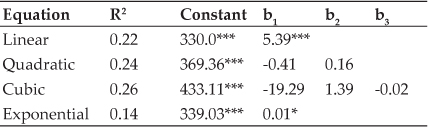
Linear model was fitted for cotton yield as there is slight deviation in value of R2 for all the models. Following graph shows the yield pattern over the years:
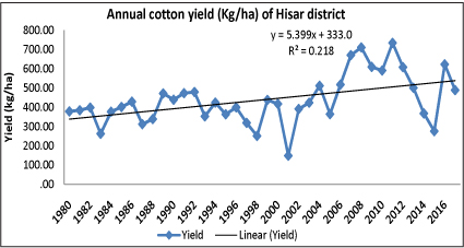
Study shows that there are ups and downs in cotton yield and linear trend has a value of R2 equal to 0.218 which is very low and graph is also showing the same. It has been observed that there is increasing trend in cotton yield during 1980-1994 and after that there is major decline in yield and it is due to incidence of insect pest and partial drought conditions. Yield gets increased after 2003 due to the evolution of Bt-Cotton but again in 2014-2016 a fall has been observed in yield due to the attack of whitefly and partial drought conditions.
In order to have complete disaggregation the whole period from 1980-81 to 2017-18 has been divided into four different sub-periods i.e. 1980-81 to 1989-90, 1990-91 to 1999-00, 2000-01 to 2009-10 and 2009-10 to 2017-18. Further, these periods have been identified as I period, II period, III period and IV period respectively. Standard deviation, mean, coefficient of variation, R2 and instability index are presented in the table 2 in these subdivided study periods:
Table 2: Summary statistics of Cotton yield of Hisar:

Mean yield of cotton is increased from 375 kg/ha in the base period to 524 kg/ha in the fourth period with an overall mean yield of 438 kg/ha. This increase is due to the adoption of high yielding varieties of cotton (Bt-Cotton) and expansion of irrigation facilities. CV is ranging between 15.8 percent to 34.7 percent with an overall variation of 29.3 percent which is reduced to 25.8 percent after the elimination of effect of trend. There is negative trend during second period that means yield of cotton decreased during second period and this reduction is due to the partial drought conditions in the state during the this period. Highest variation has been observed during third period and it is due to the evolution of Bt-Cotton and other HYV of cotton. Period four is also showing overall negative trend and variation in cotton yield as incidence of whitefly and partial drought conditions. Boxplots for the cotton yield into different study periods are also observed and given below:

Table 3: Selected Weather Yield Model for Hisar District:
Three models were fitted, model 1 is having trend yield and weather parameters as regressors, model 2 with trend yield and PC scores as regressors and third model was fitted by using trend yield and higher loading components from the component matrix as regressors.
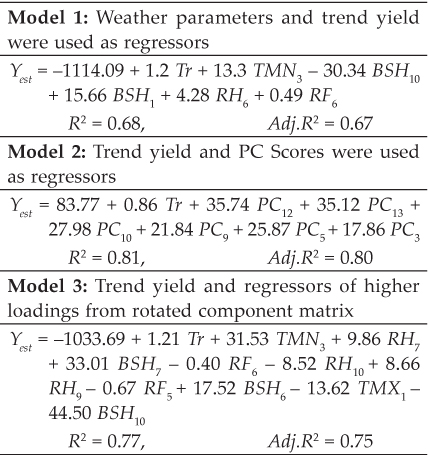
where, ϒest. - Model predicted yield (q/ha), Tr -Trend yield (kg/ha),
PC - Principal Component
TMN - Av. Minimum Temperature, TMX - Av. Maximum
Temperature
BSH - Av. Bright Sunshine Hour, RH - Av. Relative Humidity
RF - Accumulated rainfall (1, 2,..., 10/12 refer to different fortnights)
Effect of weather parameters on cotton yield
These models were fitted by using the data on cotton yield and weather parameters from 1980 to 2013. Model 1 is having trend yield and weather parameters as regressors and was developed by using stepwise regression analysis. Weather parameters have profound influence on cotton yield. Trend yield showing time effect, relative humidity and bright sunshine hours have been found major influencing factors in stepwise regression model. A rise in minimum temperature above the average minimum temperature during the 30-45 days after plantation has also been found positively correlated with cotton yield. Longer bright sunshine hours have negative impact on the yield but during the harvesting time this model can not be proposed further as it has a relatively low value of R2.
In case of model 2, PC scores and trend yield were used as regressors and yield of selected crop as response. After obtaining the PC scores a stepwise analysis was further carried out to develop the model. In all 13 PC’s were observed contributing more than 90 percent of total variation in the response. Model 2 has a relatively high value of R2 and can further be proposed. Model 2 shows that PC3, PC5, PC9, PC10, PC12 and PC13 along with trend yield are fitting the yield with higher value of R2 among all the three models.
Model 3 is using trend yield and components of higher loadings from rotated component matrix as regressors and cotton yield as response variable. Model 3 shows that if minimum temperature is below the average minimum temperature during (30-45) days after planting or vegetative stage, it affects yield positively. Rise in average maximum temperature TMX1 shows negative effective during first fifteen days (germination phase) whereas an increment in average maximum temperature TMX5 (60-75 days) is showing positive effect on flowering stage. Increased relative humidity RH7, RH9 and bright sunshine hours BSH6, BSH7, BSH9 (75-120 days) above the average, have been found beneficial during flowering stage and reproductive stage (ball formation and maturation). Increment in average Relative humidity and bright sunshine hours RH10 and BSH10 are showing negative effect hence effect could be detrimental at harvesting time.
Trend yield (Tr) is an important parameter appearing in all the models, which is an indication of technological advancement, improvement in fertilizer/insecticide/ pesticide / weedicide used and increased use of high yielding varieties.
A perusal of the results indicates the preference of using prediction equations based on principal component scores (model 2) over the regression models using weather parameters as predictor variables and higher loading model as model 2 has highest Adj-R2 followed by model 3.
The mean fortnightly maximum temperature of the study region during the cotton-growing season ranged from 45.11 to 29.22 °C and minimum temperatures have been found ranging between 14.19 to 30.26°C which is very much within the optimum temperature required for cotton growth. But sometimes, the maximum temperature exceeded 45°C and these longer duration extreme temperatures have destructive effect on cotton growth and yield. Higher RH has positive influence on crop yield but High RH also causes incidence of pest and diseases which leads to crop yield reduction. The annual average rainfall in the district is around 450 mm, out of which 133.4 and 116.2 mm is observed during July and August, respectively. The average rainfall received during normal monsoon season is 283 mm. Generally rainfall in the district increases from southwest to northeast.
Validation and comparison of the models
The performance of the forecast models has been compared on the basis of different statistics viz., Adj-R2, percent deviation of the forecast from the observed yield.
Table 4: Model Based Yield(s) along with Percent Deviations from Actual Yield(s) of Hisar District
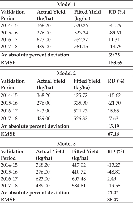
From the fitted models, cotton yield forecasts for the years 2014-15, 2015-16, 2016-17 and 2017-18 were obtained. The performance of the forecast models has been compared on the basis of different statistics viz., Adj-R2, percent deviation of the forecast from the observed yield and percent RMSE. The main reason for this performance of the developed models is incidence of whitefly on cotton for two to three years in continuation and the period of whitefly occurrence is constituted in the validation period i.e., 2014-15 and 2015-16. A perusal of the results indicates the preference of using prediction equations based on principal component scores (model 2) over the regression models using weather parameters as predictor variables and higher loading model as model 2 has highest Adj-R2 and low percent deviation of the forecast from the observed yield and percent RMSE followed by model 3.
CONCLUSION
It has been observed that there is increasing trend in cotton yield during 1980-1994 and after that there is major decline in yield and it is due to incidence of insect pest and partial drought conditions. Yield gets increased after 2003 due to the evolution of Bt-Cotton but again in 2014-2016 a fall has been observed in yield due to the attack of whitefly and partial drought conditions. Highest positive variation in cotton yield was observed during third period and it is due to the evolution of Bt-Cotton, other high yielding varieties of cotton and expansion of irrigation facilities. Three models were fitted, model 1 was having trend yield and weather parameters as regressors, model 2 with trend yield and PC scores as regressors and third model was fitted by using trend yield and higher loading components from the component matrix as regressors. A perusal of the results indicates the preference of using prediction equations based on principal component scores (model 2) over the regression models using weather parameters as predictor variables and higher loading model as model 2 has highest Adj-R2and low percent deviation of the forecast from the observed yield followed by model 3. Model 3 shows that if minimum temperature is below the average minimum temperature during (30-45) days after planting or vegetative stage, it affects yield positively. Rise in average maximum temperature TMX1 shows negative effective during first fifteen days (germination) whereas an increment in average maximum temperature TMX5 (60-75 days) is showing positive effect on flowering stage. Increased relative humidity RH7, RH9 and bright sunshine hours BSH6 BSH7, BSH9 (75-120 days) above the average, have been found beneficial during flowering stage and reproductive stage (ball formation and maturation). This study has demonstrated the utility of understanding and quantifying the relationships between cotton yield and weather variables. Trend yield (Tr) is an important parameter appearing in all the models, which is an indication of technological advancement, improvement in fertilizer/insecticide/ pesticide / weedicide used and increased use of high yielding varieties.
REFERENCES
Anderson, T.W. 1984. An Introduction to Multivariate Statistical Analysis, John Wiley & Sons Inc., New York.
Box, G.E.P. and Jenkins, G.M. 1976. Time Series Analysis: Forecasting and Control, Holden-Day, San Francisco.
Cuddy, J.D.A. and Della, V.P.A. 1978. Measuring the instability of time series data. Oxford Bull. Econ. Stat., 40(1): 79-85.
Damodar, N, Gujarti. 2003. Basic econometrics.
Debnath, M.K., Kartic Bera and Mishra, P. 2013. “Forecasting Area, Production and Yield of Cotton in India using ARIMA Model“ Research & Reviews: journal of Space Science & Technology, 1(2): 16-20.
Drapper, N.R. and Smith, H. 1998. Applied Regression Analysis. Third Edition, John and Wiley Sons, USA.
Johnson, R.A. and Wichern, D.W. 2001. Applied Multivariate Statistical Analysis, Third Edition, Prentice Hall of India Private limited, New Delhi.
Joshi, P.K., Gulati, A., Birthal, P.S. and Tewari, L. 2004. Agriculture diversification in South Asia: Patterns, determinants and policy implications. Economic and Political Weekly, 39(18): 2457-2467.
Joshi, P.K., Tewari, L. and Birthal, P.S. 2006. “Diversification and its impact on smallholders: Evidence from a study on vegetable production”. Agricultural Economics Research Review, 19(2): 219-236.
Kebebe, Ergano, Mehta, V.P. and Dixit, P.N. 2000. “Diversification of agriculture in Haryana: An empirical analysis”. Agricultural Situation in India, 57(8): 459-463.
Mishra, P., Padmanaban, K., Dhekale, B.S. and Tailor, A.K. 2018. Statistical investigation of production performance of cumin in India. Economic Affairs, 63(2): 547-555.
Mishra, P., Sahu, P.K., Dhekale, B.S. and Vishwajith K.P. 2015. “Modeling and forecasting of wheat in India and their yield Sustainability“. Society of Economics and Development, 11(3): 637-647.
Mishra, P., Sahu, P.K., Padmanaban, K., Vishwajith, K.P. and Dhekale, B.S. 2015. Study of Instability and Forecasting of Food Grain Production in India. International Journal of Agriculture Sciences, 7(3): 474-481.
Padmanaban, K., Mishra, P., Sahu, P.K. and Havaldar, Y.N. 2014. Export of cashew kernel from india: its direction and prediction. Economic Affairs, 59(4): 521.